Retirement Income Planning: Why Smart Withdrawal Strategies Matter More Than Savings
Retirement income planning isn’t just about how much you’ve saved, but about how wisely you withdraw.
This idea has spurred a new wave of retirement planning questions such as:
How much can I spend each year and not run out of money?
Instead of a fixed amount of spending annually, how does flexibility in spending impact retirement success?
How does the taxation of different investment accounts impact my after-tax spending?
How do market returns impact this on an annual basis?
The answers to these questions have created frameworks for retirees to consider when creating successful retirement outcomes.
In 1994, financial planner William Bengen introduced the “4% rule” - illustrating based on historical market conditions that retirees could withdraw 4% of their initial retirement portfolio annually, adjusted for inflation, without depleting their funds over 30 years.
In 2006, Jonathan Guyton and William Klinger expanded on the 4% by introducing dynamic withdrawal adjustments based on market conditions.
In 2010, Wade Pfau promoted a safety first approach to retirement income planning with annuities to hedge longevity risk as well as a “bucket strategy” segmenting assets into different timeframes for spending (also is a helpful psychological tool).
In 2013, Wade Pfau introduced rising equity glide paths which illustrated that starting retirement with lower equity allocations and increasing over time reduces sequence of returns risk and improves portfolio longevity.
In 2014, David Blanchett introduced the “Retirement Spending Smile” showcasing that retiree spending doesn’t remain static, rather follows a smile pattern. The idea of higher spending early in retirement for travel/hobbies, lower spending in mid-retirement as you settle into a routine, then higher spending in later years as healthcare costs rise.
In 2015, Michael Kitces found retirees often underspend due to fear of running out of money and introduced a “Ratcheting Rule” that states if a portfolio performs well, they should increase their withdrawal rate over time.
In 2020, Wade Pfau and Michael Kitces explored buffer asset strategies such as holding excess cash reserves to avoid selling stocks in downturns or using home equity lines of credit or a reverse mortgage.
There’s not a shortage of considerations to ensure you don’t run out of money in retirement.
Over the years as I’ve dug into these papers and ideas coming out of retirement planning space - I’ve found that much of these frameworks describe flexible portfolio withdrawal rate rules but lack how retirees actually pull portfolio distributions from portfolio assets.
The closest thing I’ve found is Guyton/Klinger’s capital preservation and prosperity rule which state either:
If your portfolio withdrawal rate increases by more than 20% above its original rate, then you must cut withdrawals by 10% (capital preservation rule).
If your portfolio withdrawal rate decreases by more than 20% below its original rate, then you can increase withdrawals by 10% (prosperity rule).
These rules allow for spending increases in strong markets and spending decreases in market declines - which throughout the course of a retirees life, will allow for higher lifetime spending and lower failure rates.
But the rules don’t state HOW the distributions are to be raised.
Should the distributions come from the asset allocation pro-rata? Exclusively from the equities? Exclusively from the fixed income?
I have yet to find research that expands upon this idea so I decided to build a model myself.
My hypothesis is that given two portfolios of identical asset allocation, withdrawal rates, taxes, inflation, where one portfolio pulls distributions pro-rata and the other portfolio pulls distributions exclusively either the equity or fixed income allocation based on market performance (ex: positive market = distributions from the equity allocation. Declining market = distributions from the fixed income allocation) that the portfolio that pulls dynamically based on market performance will generate a higher average ending portfolio balance.
Let’s review the assumptions:
Initial portfolio value = $1,000,000
Asset allocation = 70% stocks & 30% bonds. 80% stocks & 20% bonds. 90% stocks & 10% bonds. Where equities are U.S. large cap stocks. Where bonds are Barclays aggregate bonds.
Annual portfolio rebalancing.
Market return assumptions = 7% mean annual return for equities with a 15% standard deviation. 3% mean annual returns for bonds with a 5% standard deviation.
Returns are randomized annually through 2,000 monte carlo simulations.
Withdrawal strategy assumptions for portfolio 1 = 4% pro-rata fixed rate over time.
Withdrawal strategy assumptions for portfolio 2 = 4% pro-rata fixed rate over time. Only difference is how distributions are raised. There were three distribution options - 1 = equity only, 2 = fixed income only, 3 = pro-rata. The model was instructed to pull from the pro-rata allocation in varying percentages based on average market environments (ex: in 80% of average market environments, pull pro-rata, in 20% of top/bottom market environments, pull exclusively from fixed income or equity). Which was evaluated once per year based on the trailing 12-month returns.
Timeframe = 30 years
Taxes weren’t considered for the purpose of this analysis.
There were no inflation adjustments.
No additional contributions or expenses.
The findings of the model?
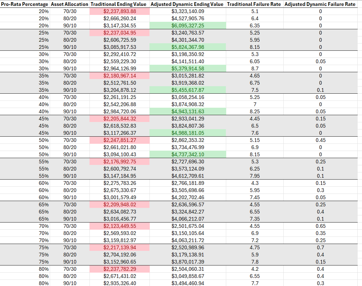

Insights I’ve drawn from this exercise are noted below:
The less the dynamic spending portfolio pulled from pro-rata, the higher the average ending balance.
Failure rates decreased with a dynamic spending approach relative to pulling exclusively from pro-rata.
Higher equity allocations benefit more from lower pro-rata withdrawals (likely from compounding interest working in favor of given higher average annualized returns).
This simulation is a little dramatic illustrating that the average difference resulted in ~$1M of ending portfolio value.
This is crazy.
While I’m not sure I fully believe the model, I think this does illustrate that in a traditional portfolio pro-rata distribution approach during bear markets selling equities leads to lower compounding potential, higher risk of being subject to sequence of returns risk, and increased failure rates.
In practice, this suggests an increased focus on where your distributions come from can potentially extend the life of your investment portfolio.